Introduction to Boosted Trees
XGBoost stands for “Extreme Gradient Boosting”, where the term “Gradient Boosting” originates from the paper Greedy Function Approximation: A Gradient Boosting Machine, by Friedman.
The term gradient boosted trees has been around for a while, and there are a lot of materials on the topic. This tutorial will explain boosted trees in a self-contained and principled way using the elements of supervised learning. We think this explanation is cleaner, more formal, and motivates the model formulation used in XGBoost.
Elements of Supervised Learning
XGBoost is used for supervised learning problems, where we use the training data (with multiple features) \(x_i\) to predict a target variable \(y_i\). Before we learn about trees specifically, let us start by reviewing the basic elements in supervised learning.
Model and Parameters
The model in supervised learning usually refers to the mathematical structure of by which the prediction \(y_i\) is made from the input \(x_i\). A common example is a linear model, where the prediction is given as \(\hat{y}_i = \sum_j \theta_j x_{ij}\), a linear combination of weighted input features. The prediction value can have different interpretations, depending on the task, i.e., regression or classification. For example, it can be logistic transformed to get the probability of positive class in logistic regression, and it can also be used as a ranking score when we want to rank the outputs.
The parameters are the undetermined part that we need to learn from data. In linear regression problems, the parameters are the coefficients \(\theta\). Usually we will use \(\theta\) to denote the parameters (there are many parameters in a model, our definition here is sloppy).
Objective Function: Training Loss + Regularization
With judicious choices for \(y_i\), we may express a variety of tasks, such as regression, classification, and ranking. The task of training the model amounts to finding the best parameters \(\theta\) that best fit the training data \(x_i\) and labels \(y_i\). In order to train the model, we need to define the objective function to measure how well the model fit the training data.
A salient characteristic of objective functions is that they consist of two parts: training loss and regularization term:
where \(L\) is the training loss function, and \(\Omega\) is the regularization term. The training loss measures how predictive our model is with respect to the training data. A common choice of \(L\) is the mean squared error, which is given by
Another commonly used loss function is logistic loss, to be used for logistic regression:
The regularization term is what people usually forget to add. The regularization term controls the complexity of the model, which helps us to avoid overfitting. This sounds a bit abstract, so let us consider the following problem in the following picture. You are asked to fit visually a step function given the input data points on the upper left corner of the image. Which solution among the three do you think is the best fit?
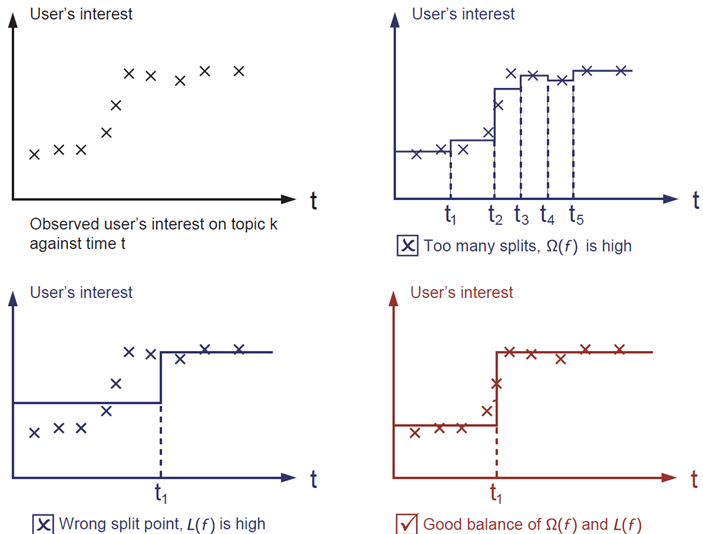
The correct answer is marked in red. Please consider if this visually seems a reasonable fit to you. The general principle is we want both a simple and predictive model. The tradeoff between the two is also referred as bias-variance tradeoff in machine learning.
Why introduce the general principle?
The elements introduced above form the basic elements of supervised learning, and they are natural building blocks of machine learning toolkits. For example, you should be able to describe the differences and commonalities between gradient boosted trees and random forests. Understanding the process in a formalized way also helps us to understand the objective that we are learning and the reason behind the heuristics such as pruning and smoothing.
Decision Tree Ensembles
Now that we have introduced the elements of supervised learning, let us get started with real trees. To begin with, let us first learn about the model choice of XGBoost: decision tree ensembles. The tree ensemble model consists of a set of classification and regression trees (CART). Here’s a simple example of a CART that classifies whether someone will like a hypothetical computer game X.
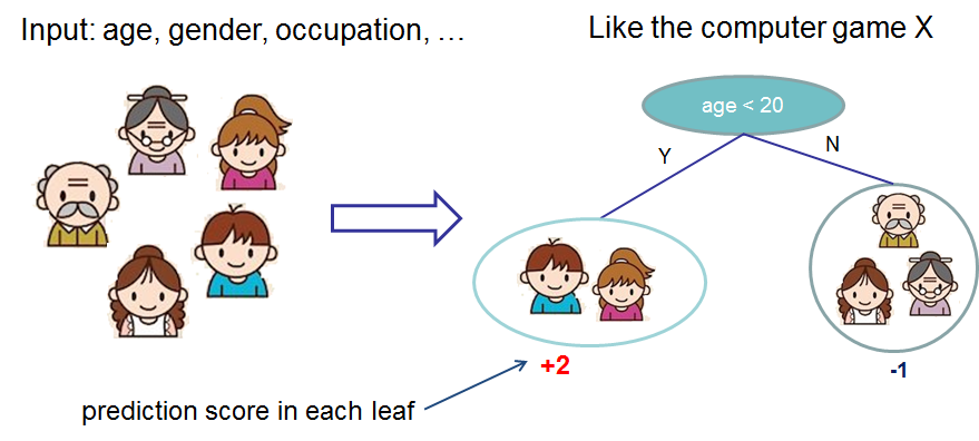
We classify the members of a family into different leaves, and assign them the score on the corresponding leaf. A CART is a bit different from decision trees, in which the leaf only contains decision values. In CART, a real score is associated with each of the leaves, which gives us richer interpretations that go beyond classification. This also allows for a principled, unified approach to optimization, as we will see in a later part of this tutorial.
Usually, a single tree is not strong enough to be used in practice. What is actually used is the ensemble model, which sums the prediction of multiple trees together.
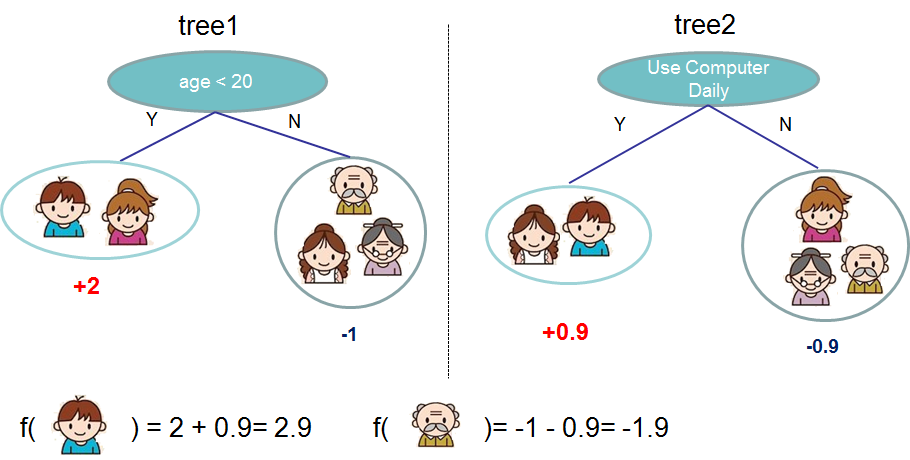
Here is an example of a tree ensemble of two trees. The prediction scores of each individual tree are summed up to get the final score. If you look at the example, an important fact is that the two trees try to complement each other. Mathematically, we can write our model in the form
where \(K\) is the number of trees, \(f_k\) is a function in the functional space \(\mathcal{F}\), and \(\mathcal{F}\) is the set of all possible CARTs. The objective function to be optimized is given by
where \(\omega(f_k)\) is the complexity of the tree \(f_k\), defined in detail later.
Now here comes a trick question: what is the model used in random forests? Tree ensembles! So random forests and boosted trees are really the same models; the difference arises from how we train them. This means that, if you write a predictive service for tree ensembles, you only need to write one and it should work for both random forests and gradient boosted trees. (See Treelite for an actual example.) One example of why elements of supervised learning rock.
Tree Boosting
Now that we introduced the model, let us turn to training: How should we learn the trees? The answer is, as is always for all supervised learning models: define an objective function and optimize it!
Let the following be the objective function (remember it always needs to contain training loss and regularization):
in which \(t\) is the number of trees in our ensemble. (Each training step will add one new tree, so that at step \(t\) the ensemble contains \(K=t\) trees).
Additive Training
The first question we want to ask: what are the parameters of trees? You can find that what we need to learn are those functions \(f_k\), each containing the structure of the tree and the leaf scores. Learning tree structure is much harder than traditional optimization problem where you can simply take the gradient. It is intractable to learn all the trees at once. Instead, we use an additive strategy: fix what we have learned, and add one new tree at a time. We write the prediction value at step \(t\) as \(\hat{y}_i^{(t)}\). Then we have
It remains to ask: which tree do we want at each step? A natural thing is to add the one that optimizes our objective.
If we consider using mean squared error (MSE) as our loss function, the objective becomes
The form of MSE is friendly, with a first order term (usually called the residual) and a quadratic term. For other losses of interest (for example, logistic loss), it is not so easy to get such a nice form. So in the general case, we take the Taylor expansion of the loss function up to the second order:
where the \(g_i\) and \(h_i\) are defined as
After we remove all the constants, the specific objective at step \(t\) becomes
This becomes our optimization goal for the new tree. One important advantage of this definition is that the value of the objective function only depends on \(g_i\) and \(h_i\). This is how XGBoost supports custom loss functions. We can optimize every loss function, including logistic regression and pairwise ranking, using exactly the same solver that takes \(g_i\) and \(h_i\) as input!
Model Complexity
We have introduced the training step, but wait, there is one important thing, the regularization term! We need to define the complexity of the tree \(\omega(f)\). In order to do so, let us first refine the definition of the tree \(f(x)\) as
Here \(w\) is the vector of scores on leaves, \(q\) is a function assigning each data point to the corresponding leaf, and \(T\) is the number of leaves. In XGBoost, we define the complexity as
Of course, there is more than one way to define the complexity, but this one works well in practice. The regularization is one part most tree packages treat less carefully, or simply ignore. This was because the traditional treatment of tree learning only emphasized improving impurity, while the complexity control was left to heuristics. By defining it formally, we can get a better idea of what we are learning and obtain models that perform well in the wild.
The Structure Score
Here is the magical part of the derivation. After re-formulating the tree model, we can write the objective value with the \(t\)-th tree as:
where \(I_j = \{i|q(x_i)=j\}\) is the set of indices of data points assigned to the \(j\)-th leaf. Notice that in the second line we have changed the index of the summation because all the data points on the same leaf get the same score. We could further compress the expression by defining \(G_j = \sum_{i\in I_j} g_i\) and \(H_j = \sum_{i\in I_j} h_i\):
In this equation, \(w_j\) are independent with respect to each other, the form \(G_jw_j+\frac{1}{2}(H_j+\lambda)w_j^2\) is quadratic and the best \(w_j\) for a given structure \(q(x)\) and the best objective reduction we can get is:
The last equation measures how good a tree structure \(q(x)\) is.
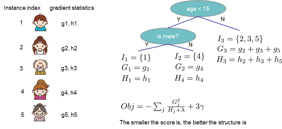
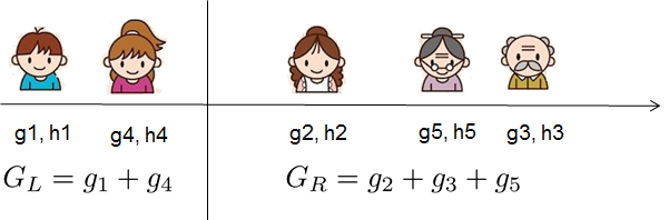
If all this sounds a bit complicated, let’s take a look at the picture, and see how the scores can be calculated. Basically, for a given tree structure, we push the statistics \(g_i\) and \(h_i\) to the leaves they belong to, sum the statistics together, and use the formula to calculate how good the tree is. This score is like the impurity measure in a decision tree, except that it also takes the model complexity into account.
Learn the tree structure
Now that we have a way to measure how good a tree is, ideally we would enumerate all possible trees and pick the best one. In practice this is intractable, so we will try to optimize one level of the tree at a time. Specifically we try to split a leaf into two leaves, and the score it gains is
This formula can be decomposed as 1) the score on the new left leaf 2) the score on the new right leaf 3) The score on the original leaf 4) regularization on the additional leaf. We can see an important fact here: if the gain is smaller than \(\gamma\), we would do better not to add that branch. This is exactly the pruning techniques in tree based models! By using the principles of supervised learning, we can naturally come up with the reason these techniques work :)
For real valued data, we usually want to search for an optimal split. To efficiently do so, we place all the instances in sorted order, like the following picture.
A left to right scan is sufficient to calculate the structure score of all possible split solutions, and we can find the best split efficiently.
Note
Limitation of additive tree learning
Since it is intractable to enumerate all possible tree structures, we add one split at a time. This approach works well most of the time, but there are some edge cases that fail due to this approach. For those edge cases, training results in a degenerate model because we consider only one feature dimension at a time. See Can Gradient Boosting Learn Simple Arithmetic? for an example.
Final words on XGBoost
Now that you understand what boosted trees are, you may ask, where is the introduction for XGBoost? XGBoost is exactly a tool motivated by the formal principle introduced in this tutorial! More importantly, it is developed with both deep consideration in terms of systems optimization and principles in machine learning. The goal of this library is to push the extreme of the computation limits of machines to provide a scalable, portable and accurate library. Make sure you try it out, and most importantly, contribute your piece of wisdom (code, examples, tutorials) to the community!